Understanding Systems Factorial Technology (SFT)
Introduction
On the corner of a busy road, a man waits for the lights to change. Impatient to be home, he looks down at his phone and replies to a message. Glimpsing a green signal and hearing the crossing buzz, he steps out onto the road.
Our experience of the world relies upon the independent processing and seamless integration of sensory modalities. Tactile, auditory, olfactory and visual information all combine to provide a rich description of the world around us. In the above example, visual cues --- the flash of green --- and auditory cues --- the buzzing signal --- are integrated simultaneously to reach a decisions. This everyday example frames an important question for cognitive scientists: How do we unify two independent sensory streams into a single conscious experience? The following provides a brief history of response-time models in cognitive psychology and how response-time can be used to answer this complex question.
Cognitive Architecture
Since Donders' (1868) subtraction method, cognitive scientists have been using response times (RT) to measure cognitive processes. Donder's assumed that RT could act to measure the additive cognitive processes that underlie behaviour. For example, the cognitive processes of seeing a green light and deciding to walk. By measuring each component in isolation, and subtracting their response-times, Donder's created a measure of cognitive processing.
A key assumption of Donder's work was that cognitive processes were additive. A process is additive when the total decision time is equal to the sum of each component processes. Today, additive cognitive processes go by another name, a serial processing system. Under a serial processing system, each component process must terminate before the next may begin. For example, a green walk signal must finish being processed before an auditory buzz may be evaluated. Although serial systems are necessary for many tasks, for example, one must see an object before picking it up; many cognitive process occur simultaneously in a parallel processing system.
Egeth (1966) was the first to use RTs to differentiate parallel from serial processing systems. Egeth assumed that if all items within an array were processes simultaneously, (i.e., in parallel), the addition of further items would have no impact on decision-time. As such, a parallel system would predict a flat mean RT slope over increasing array sizes. By contrast, a serial system would predict a steep mean RT slope, increasing with arrays size.
As an early adopter of this method, Sternberg (1966) applied these principles to examine whether short-term memory was accessed in serial or in parallel. In his task, participants were presented a list of digits followed by a probe, and were asked to report whether the probed digit was in the memory list. Sternberg found that response-times increased linearly with the length of the memory list. This additivity was used as evidence of a serial processing system, a claim propagated by many influential studies (e.g., Sternberg, 1969; Cohen, 1973; Shiffrin, 1977; Navon, 1977}, and none more influential than Treisman & Gelade (1980).
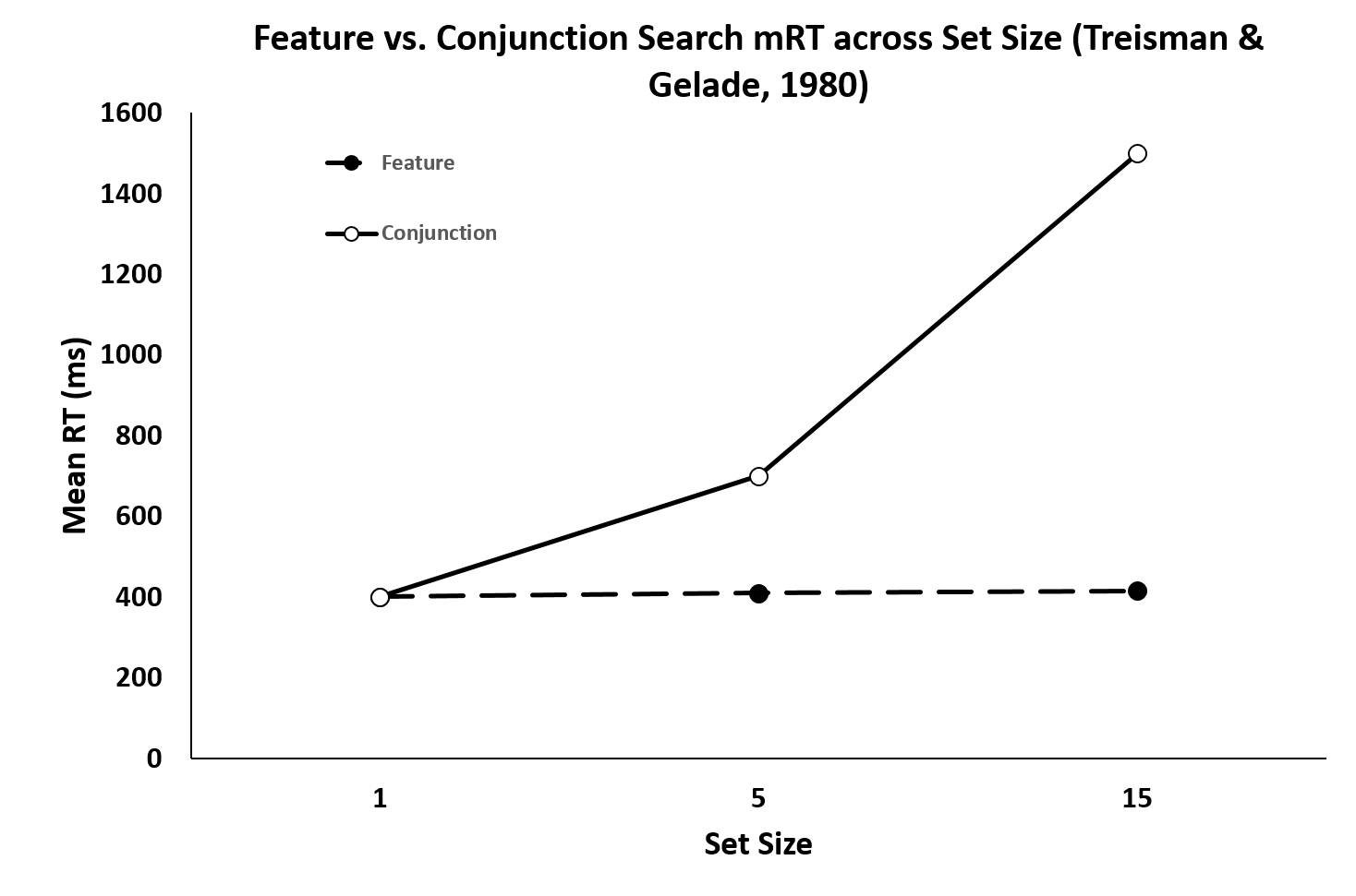
In their 1980 Feature Integration Theory of Attention, Treisman and Gelade used mean RT to differentiate parallel and serial visual processing systems. They found RT was invariant across set size when participants searched a display for a singular feature (a dimension of a stimulus, such as a colour or shape), however, increased monotonicity when searching for a conjunction of features (i.e., a coloured triangle; see Figure 1). These findings suggest that a singular feature could be processed irrespective of set size, through a parallel (or over-additive) cognitive processing system. Although compelling, the findings of Treisman and Gelade ignored a key component of a system processing: efficiency.
Workload capacity
Processing efficiency or workload capacity describes the rate at which information may pass through a processing system. Workload capacity is intimately tied to the processing architecture (parallel vs serial) of a system at the mean response-time level, often resulting in the phenomenon of model mimicry. Model mimicry describes how a slow, inefficient parallel system may produce identical mean response-times as a faster serial system. The efficiency of a processing system may be described as either limited, unlimited or super in workload capacity.
A limited workload capacity system slows with additional sources of information, for example, processing a green walk sign in the presence of an additional buzzing signal. An unlimited workload capacity system is unaffected by additional sources of information, and a super-capacity system speeds up with additional sources of information. The mean RT predictions of Treisman and Gelade (1980) and colleagues were formed under the assumption of unlimited workload capacity. More recent work has since thrown these assumptions into question (Townsend, 1989; 1071; 1977; 1995; 2004; Eidels et al., 2010; Houpt, 2012; Houpt et al., 2014; Garrett et al., 2018). To address the problem of model mimicry, James Townsend and colleagues (Townsend et al., 1995; 2004; 2011) have developed a theoretically driven framework and suit of mathematical tools, known as Systems Factorial Technology (SFT).
Systems Factorial Technology
SFT is a theoretical framework, augmented by experimental methodology, that uses response-time distributions to generate unique system-models. By comparing these theoretical models to experimental data, SFT is able to identify system properties without the confound of model mimicry. Specifically, SFT was designed to identify and assess the system properties of architecture, workload capacity, stopping-rule and channel (in)dependence.
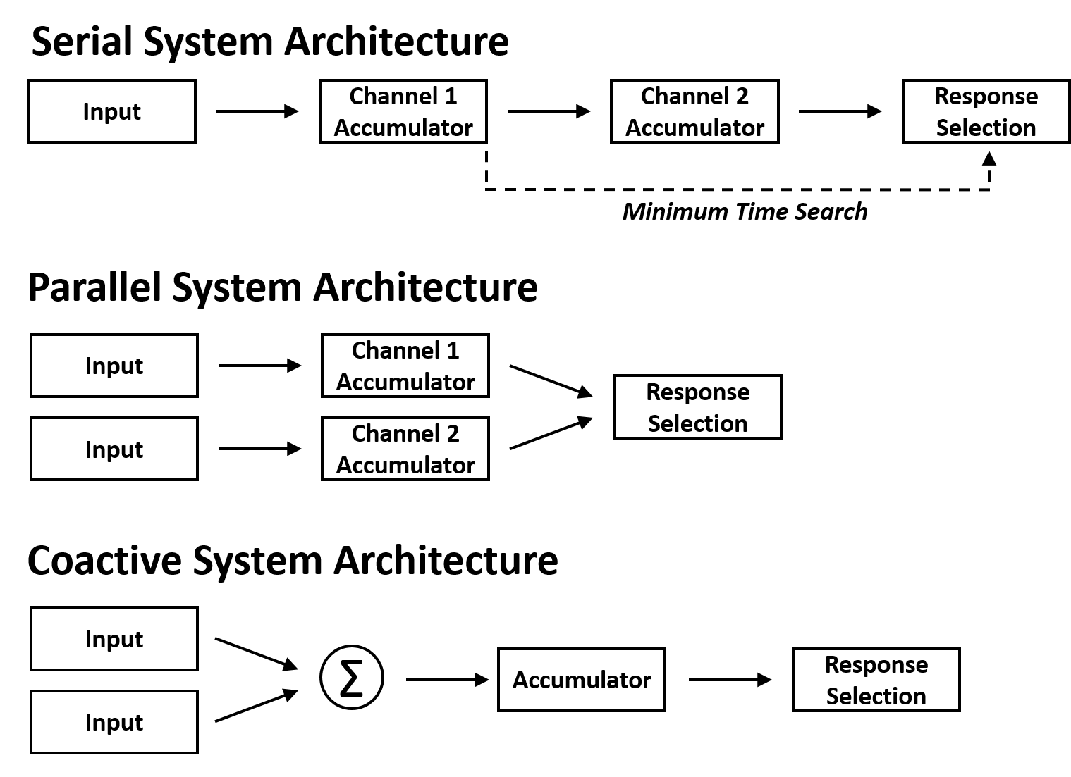
Architecture describes the time-course at which information channels are combined (parallel vs serial) and workload capacity describes the system efficiency (limited, unlimited and super). Stopping-rule describes how and when processing may terminate. A self-terminating or minimum-time stopping-rule may terminate before all sources of information are fully processed (e.g., you may terminate your search for a cookie at the moment of its detection). An exhaustive or maximum-time stopping-rule must process all sources of information before a decision can be reached (e.g., you must check all the cookie's ingredients for your friend's nut allergy; see Figure 2). Finally, channel (in)dependence describes whether information channels are stochastically separate. Independent channels provide no information to one-another. Dependent channels share information and may act to facilitate or inhibit the decision process (see Eidels et al., 2011). A coactive model describes a special case of parallel processing, where information channels sum together to reach a decision. Notably, a coactive model is unaffected by stopping-rule and predicts super workload capacity.
SFT is both an analysis tool set and methodological framework. SFT uses distributional analysis tools to directly assess the properties of system architecture, stopping-rule and workload capacity, under the assumption of channel independence. These analysis tools require a specific methodological design, termed the double-factorial redundant-target paradigm (DFP).
The Double Factorial Paradigm
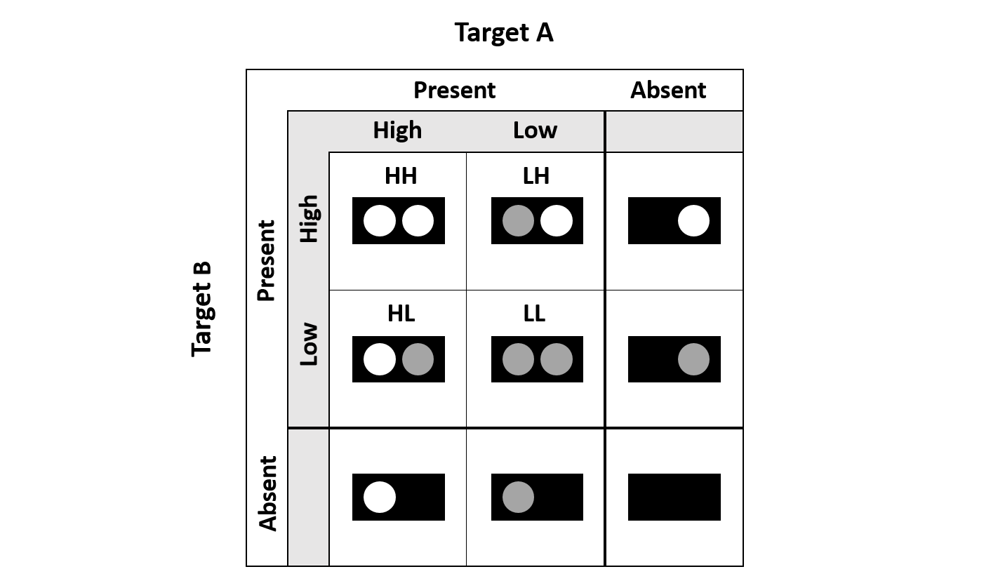
Figure 3 illustrates a prototypical DFP using a dot-detection task. Here, a target is defined by any source of light, and may appear in the left (channel A) or right (channel B) location. Load, (i.e., the number of information channels), is manipulated by the presence or absence of a target. Within the target conditions exists a second manipulation of target salience, (i.e., target discriminability). A high salience (H) target is easier and faster to respond to than a low salience (L) target. Double-target cells are redundant, as either target would constitute a correct `target present' response. Together, these redundant-cells host four combinations of double-target salience: high-high (HH), high-low (HL), low-high (LH) and low-low (LL). The combined manipulation of load (target presence vs absence) and salience (discriminability high vs low) allows the specially designed analysis tools of SFT to perform independent assessments of system workload and processing architecture.
The Capacity Coefficient
The first factorial manipulation of load allows for calculation of the capacity coefficient C(t). The capacity coefficient measures the change in efficiency of the processing system as workload, (i.e., the number of information channels), increases. The capacity coefficient is calculated by comparing the response-time distribution for double-target trials, to the response-time distribution for trials when a target is present in each channel alone --- single-target trials. Formally, the capacity coefficient is expressed as:
C(t) = log(sAB(t)) / [log(sA(t)) + log(sB(t))]
where letters A and B refer to the processing channels when each channel operates alone, A or B, or together AB. S(t) refers to the survivor function of the channel response-times, t is time, and log is the natural logarithm. The measured change in efficiency between the channel conditions is evaluated against predictions derived from an unlimited capacity independent parallel (UCIP) model. Under the UCIP benchmark model, an unlimited capacity system predicts C(t) = 1. A super capacity system, one that speeds with additional workload, predicts C(t) > 1. Finally, a limited capacity system predicts C(t) < 1.
The Mean Interaction Contrast
The second factorial manipulation, that of target salience, allows for diagnosis of the system processing architecture through two measures: the mean interaction contrast and the survivor interaction contrast. The mean interaction contrast or MIC, is calculated as a double-difference of mean RT between the four factorial combinations of salience. Formally, the MIC may be written as:
MIC = mHH - mHL - mLH + mLL
where m denotes a mean response-time, and the letters H and L denote the display salience as combinations of high (H; i.e., bright dot) and low (L; i.e., dull dot) double-target salience-conditions. Thus, HH indicates a trial with two salient targets (two bright dots), HL and LH indicate a trial with one salient and one dull target item, and LL indicates a trial with two dull target items. As high salience targets should be responded to faster than low-salience targets, correct MIC interpretation requires the following ordering: mHH < mHL, mLH < mLL. Under the assumption of a UCIP model, and correct ordering of the mean RTs, a parallel minimum-time model predicts an over-additive MIC > 0, a parallel maximum-time model predicts an under-additive MIC < 0 and all serial models predict an additive MIC = 0. These three predictions allow the MIC to easily differentiate between parallel and serial models. To further diagnose stopping-rule, we must turn to the survivor interaction contrast (SIC).
The Survivor Interaction Contrasts
The SIC is a contrast measure, similar to the MIC, but calculated from the survivor functions of each double-target salience combination. It is defined as:
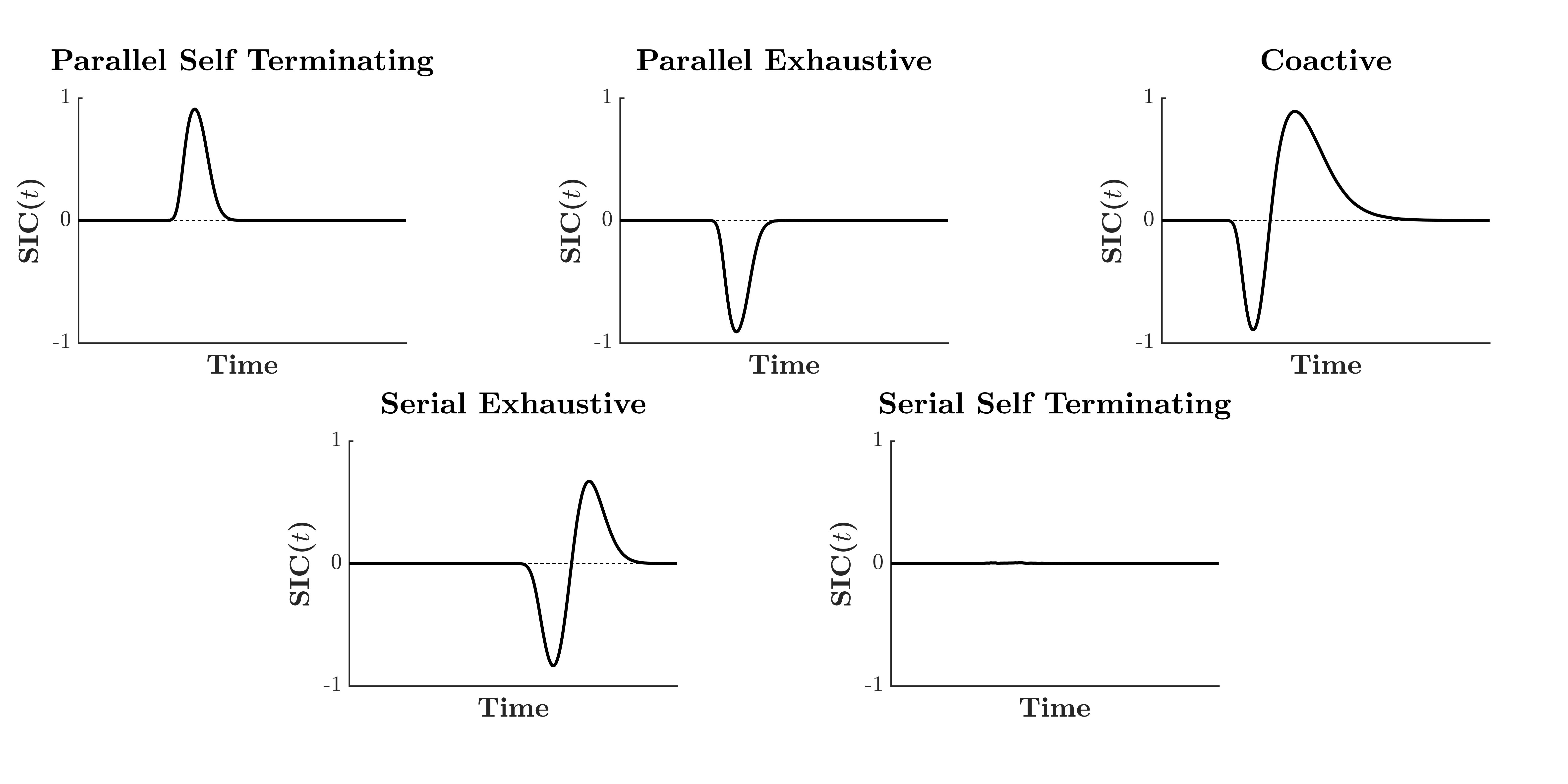
SIC(t) = sHH(t) - sHL(t) - sLH(t) + sLL(t)
Different models predict unique SIC(t) functions, as illustrated in Figure 4. A necessary assumption for valid interpretation of the SICSIC(t) is the assumption of selective influence and ordering of the composite salience conditions such that sHH(t) < sHL(t), sLH(t) < sLL(t). Fortunately, these survivor functions are easily subjected to non-parametric tests. Appropriate application of the SIC(t) and MIC allows for comprehensive diagnosis of system architecture and stopping rule within the double-target condition.
By combining the distributional system measures of SFT, specifically the SIC(t) and C(t), Systems Factorial Technology is able to independently diagnose processing architecture, stopping-rule and workload capacity without the confound of model mimicry.
Understanding SFT and the system tools therein is difficult for new scientists. To help with this process, an introductory paper titled SFT explained to humans have been written, and an R package has been created by Joe Houpt. To further assist in this process, I have also created a small SFT in Matlab package that provides functions to generate simulations, analyse and plot SFT data (e.g., Figure 4). The section 'SFT in Matlab' will detail these efforts (tba).